Open and analyse shoot output netcdf

import cartopy.crs as ccrs
import cmocean as cm
import matplotlib.pyplot as plt
import numpy as np
import xarray as xr

from shoot.num import points_in_polygon
from shoot.plot import create_map, pcarr
from shoot.samples import get_sample_file

pmerc = ccrs.Mercator()

Usefull function

def create_map_ax(
    lons,
    lats,
    ax,
    margin=0.0,
    square=False,
    coastlines=True,
    emodnet=False,
    title=None,
    **kwargs,
):
    """Create a simple decorated cartopy map"""
    # lons, lats = lons.values, lats.values
    xmin, xmax = np.min(lons), np.max(lons)
    ymin, ymax = np.min(lats), np.max(lats)
    dx, dy = xmax - xmin, ymax - ymin
    x0, y0 = 0.5 * (xmin + xmax), 0.5 * (ymin + ymax)
    if square:
        aspect = dx / dy * np.cos(np.radians(y0))
        if aspect > 1:
            dy *= aspect
        else:
            dx /= aspect
    xmargin = margin * dx
    ymargin = margin * dy
    xmin = x0 - 0.5 * dx - xmargin
    xmax = x0 + 0.5 * dx + xmargin
    ymin = y0 - 0.5 * dy - ymargin
    ymax = y0 + 0.5 * dy + ymargin

    ax.set_extent([xmin, xmax, ymin, ymax])
    ax.gridlines(
        draw_labels=["bottom", "left"],
        linewidth=1,
        color="k",
        alpha=0.5,
        linestyle="--",
        rotate_labels=False,
    )
    if coastlines:
        ax.coastlines()
    if emodnet:
        ax.add_wms("https://ows.emodnet-bathymetry.eu/wms", "emodnet:mean_atlas_land")
    if title:
        ax.set_title(title)
    return fig, ax

Initialisation

#  Import data

root_path = "OBS/SATELLITE/jan2024_ionian_sea_duacs.nc"
path = get_sample_file(root_path)
ds = xr.open_dataset(path)
root_track = "EDDIES/track_ionian_sea_duacs_jan2024.nc"
track_path = get_sample_file(root_track)
tracks = xr.open_dataset(track_path)
tracks

<xarray.Dataset> Size: 1MB
Dimensions:               (obs: 820, nb_sample: 50, eddies: 71)
Dimensions without coordinates: obs, nb_sample, eddies
Data variables: (12/30)
    time                  (obs) datetime64[ns] 7kB ...
    i_cen                 (obs) int64 7kB ...
    j_cen                 (obs) int64 7kB ...
    x_cen                 (obs) float64 7kB ...
    y_cen                 (obs) float64 7kB ...
    track_id              (obs) int64 7kB ...
    ...                    ...
    life_time             (eddies) float64 568B ...
    x_start               (eddies) float64 568B ...
    y_start               (eddies) float64 568B ...
    x_end                 (eddies) float64 568B ...
    y_end                 (eddies) float64 568B ...
    eddy_type             (eddies) <U11 3kB ...
Attributes:
    window_center:  50 km
    window_fit:     120 km
    min_radius:     20 km
    project:        SHOOT
    institution:    SHOM
    contact:        jean.baptiste.roustan@shom.fr

Plots

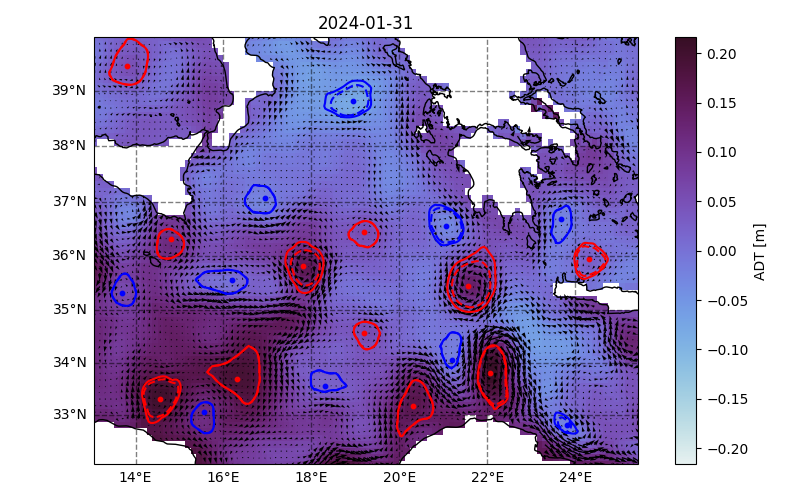
# Plot tracking

fig, ax = create_map(ds.longitude, ds.latitude, figsize=(8, 5))
colors = {"cyclone": "b", "anticyclone": "r"}

dss = ds.isel(time=-1)

cb = dss.adt.plot(
    x="longitude",
    y="latitude",
    cmap="cmo.dense",
    ax=ax,
    add_colorbar=False,
    transform=pcarr,
)

plt.colorbar(cb, label="ADT [m]")

nj = 1
plt.quiver(
    dss.longitude[::nj].values,
    dss.latitude[::nj].values,
    dss.ugos[::nj, ::nj].values,
    dss.vgos[::nj, ::nj].values,
    transform=pcarr,
)


day = np.where(tracks.time.values == dss.time.values)[0]
track_day = tracks.isel(obs=day)

for i in range(len(track_day.obs)):
    tmp = track_day.isel(obs=i)
    plt.scatter(
        tmp.x_cen,
        tmp.y_cen,
        c=colors[str(tmp.eddy_type.isel(eddies=tmp.track_id.values).values)],
        s=10,
        transform=pcarr,
    )

    plt.plot(
        tmp.x_vmax_contour,
        tmp.y_vmax_contour,
        "--",
        c=colors[str(tmp.eddy_type.isel(eddies=tmp.track_id.values).values)],
        transform=pcarr,
    )

    plt.plot(
        tmp.x_eff_contour,
        tmp.y_eff_contour,
        c=colors[str(tmp.eddy_type.isel(eddies=tmp.track_id.values).values)],
        transform=pcarr,
    )

plt.title(np.datetime_as_string(dss.time, unit="D"))
plt.tight_layout()

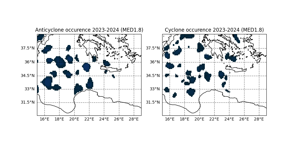
#### Heatmaps

## to be modified by the user
lons = np.arange(-6, 36, 0.1)
lats = np.arange(30, 44.5, 0.1)

count_s_anti = np.zeros((len(lats), len(lons)))
count_s_cyc = np.zeros((len(lats), len(lons)))

ind_anti = np.where(tracks.eddy_type[tracks.track_id.values].values == "anticyclone")[0]
ind_cyc = np.where(tracks.eddy_type[tracks.track_id.values].values == "cyclone")[0]

shoot_anti = tracks.isel(obs=ind_anti)
shoot_cyc = tracks.isel(obs=ind_cyc)

## Should work with previously made modifications

Xlons, Xlats = np.meshgrid(lons, lats)


for i in range(len(shoot_anti.obs)):
    line = np.array(
        [
            shoot_anti.isel(obs=i).x_vmax_contour,
            shoot_anti.isel(obs=i).y_vmax_contour,
        ]
    ).T
    for j in range(len(lons)):  # On parcoure le tableau via les longitude
        points = np.array([Xlons[:, j], Xlats[:, j]]).T
        in_poly = points_in_polygon(points, line)
        # print(in_poly)
        count_s_anti[:, j] += in_poly

for i in range(len(shoot_cyc.obs)):
    line = np.array(
        [
            shoot_cyc.isel(obs=i).x_vmax_contour,
            shoot_cyc.isel(obs=i).y_vmax_contour,
        ]
    ).T
    for j in range(len(lons)):  # On parcoure le tableau via les longitude
        points = np.array([Xlons[:, j], Xlats[:, j]]).T
        in_poly = points_in_polygon(points, line)
        # print(in_poly)
        count_s_cyc[:, j] += in_poly


count_s_anti[count_s_anti == 0] = np.nan
count_s_cyc[count_s_cyc == 0] = np.nan


fig, axs = plt.subplots(1, 2, subplot_kw=dict(projection=pmerc), figsize=(10, 5))
# create_map_ax(np.arange(-6, 36), np.arange(30, 44.5), axs[0])
create_map_ax(np.arange(15, 30), np.arange(30, 40), axs[0])
plt.sca(axs[0])
plt.title("Anticyclone occurence 2023-2024 (MED1.8)")
plt.pcolormesh(
    lons,
    lats,
    count_s_anti / 510,
    transform=pcarr,
    vmin=0,
    vmax=0.7,
    cmap=cm.cm.thermal,
)

# create_map_ax(np.arange(-6, 36), np.arange(30, 44.5), axs[1])
create_map_ax(np.arange(15, 30), np.arange(30, 40), axs[1])
plt.sca(axs[1])
plt.title("Cyclone occurence 2023-2024 (MED1.8)")
plt.pcolormesh(
    lons,
    lats,
    count_s_cyc / 510,
    transform=pcarr,
    vmin=0,
    vmax=0.7,
    cmap=cm.cm.thermal,
)

<cartopy.mpl.geocollection.GeoQuadMesh object at 0x70269b43de90>