Detect CROCO-GIGATL1 eddies at 1000m

In this example, eddies are detected from CROCO model currents interpolated to 1000 m and collocated at RHO points.

Initialisations

Import needed stuff.

import time

import cmocean as cm
import matplotlib.pyplot as plt
import xarray as xr

from shoot.dyn import get_relvort
from shoot.eddies.eddies2d import Eddies2D
from shoot.meta import set_meta_specs
from shoot.plot import create_map, pcarr
from shoot.samples import get_sample_file

xr.set_options(display_style="text")

<xarray.core.options.set_options object at 0x7026ac9b6dd0>

Read data

# Mind that the dataarray should be 2D : single time and single depth
set_meta_specs("croco")
root_path = "MODELS/CROCO/GIGATL/gigatl1-1000m.nc"
path = get_sample_file(root_path)
ds = xr.open_dataset(path).isel(time=0)

Detect eddies

Parameters

Window size in km to compute the LNAM and find eddy centers

window_center = 50

Window size in km to fit SSH and make other diagnostics like contours

window_fit = 120

Minimal radius of an eddy to retain it

min_radius = 10

Ellipse error preconised 1% for deep field, 5% to 10% to surface field

ellipse_error = 0.02

Detection

start = time.time()
eddies = Eddies2D.detect_eddies(
    ds.u,
    ds.v,
    window_center,
    window_fit=window_fit,
    min_radius=min_radius,
    paral=False,
    ellipse_error=ellipse_error,
)
end = time.time()
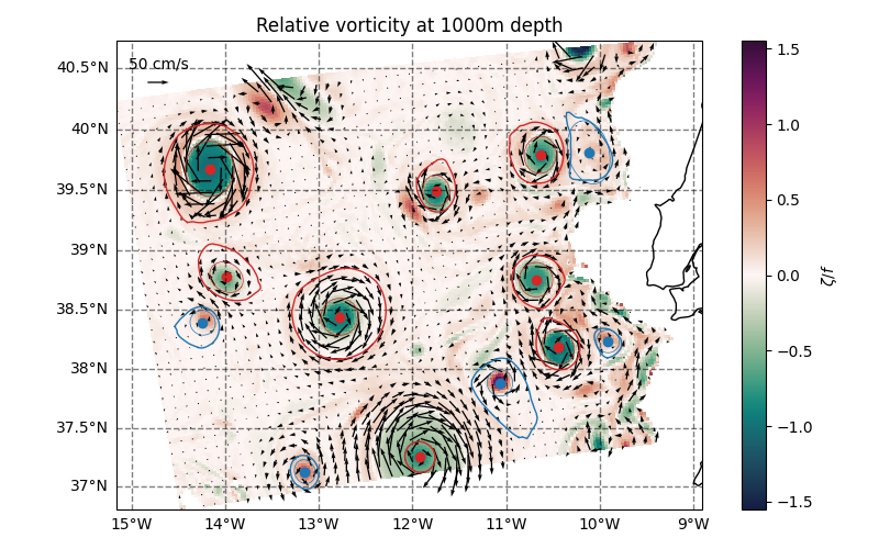
print(f"Number of detected eddies {len(eddies.eddies)} in {end - start:.1f} s")

Number of detected eddies 13 in 38.6 s

Plots

We plot eddies with the relative vorticity as background.

fig, ax = create_map(ds.lon_rho, ds.lat_rho, figsize=(8, 5))
vort = get_relvort(ds.u, ds.v) / 1e-4
cb = vort.plot(
    x="lon_rho",
    y="lat_rho",
    cmap=cm.cm.curl,
    ax=ax,
    add_colorbar=False,
    transform=pcarr,
)
plt.colorbar(cb, label=r"$\zeta/f$")
nj = 4
qv = plt.quiver(
    ds.lon_rho[::nj, ::nj].values,
    ds.lat_rho[::nj, ::nj].values,
    ds.u[::nj, ::nj].values,
    ds.v[::nj, ::nj].values,
    transform=pcarr,
)
plt.quiverkey(qv, 0.18, 0.85, 0.5, "50 cm/s", coordinates='figure')

for eddy in eddies.eddies:
    eddy.plot(transform=pcarr, lw=1, boundary=True)
plt.title("Relative vorticity at 1000m depth")
plt.tight_layout()