Profile anomalies diags

This example requires 3D dataset including depth dimension Hydrology anomalies can be performes in every 3D fields.

Initialisations

Import needed stuff.

import time

import cmocean as cm
import matplotlib.pyplot as plt
import xarray as xr

from shoot.dyn import get_relvort
from shoot.eddies.eddies2d import Eddies2D
from shoot.hydrology import Anomaly, compute_anomalies
from shoot.meta import set_meta_specs
from shoot.plot import create_map, pcarr
from shoot.samples import get_sample_file

xr.set_options(display_style="text")

<xarray.core.options.set_options object at 0x7026857d2b10>

Read data

set_meta_specs("croco")
root_path = "MODELS/CROCO/MED/pelops_3d.nc"
path = get_sample_file(root_path)
ds_3d = xr.open_dataset(path)
ds_2d = ds_3d.isel(s_rho=len(ds_3d.s_rho) - 1)

Detect eddies

Parameters

window_center = 50

window_fit = 120

min_radius = 10

ellipse_error = 0.05

Detection

start = time.time()

eddies = Eddies2D.detect_eddies(
    ds_2d.u,
    ds_2d.v,
    window_center,
    window_fit=window_fit,
    ssh=ds_2d.zeta,
    min_radius=min_radius,
    paral=True,
)
end = time.time()
print("it takes %.1f s" % (end - start))

it takes 3.0 s

Anomalies

# Detect anomaly exemple on a particular eddy
# ~~~~~~~~~~~~~~~~~~~~~~~~~~~~~~~~~~~~~~~~~~~


eddy = eddies.eddies[0]
# here you can choose the desire variable : density, salinity, temp, celerity
anomaly = Anomaly(eddy, eddies, ds_3d.sig0, depth=ds_3d.depth, r_factor=1.2)

Plots

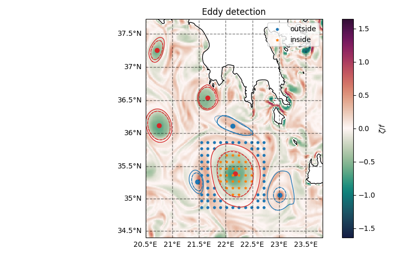
We plot eddies with the relative vorticity as background. It shows the selected inside and outside profiles

fig, ax = create_map(ds_2d.lon_rho, ds_2d.lat_rho, figsize=(8, 5))
vort = get_relvort(ds_2d.u, ds_2d.v) / 1e-4
cb = vort.plot(
    x="lon_rho",
    y="lat_rho",
    cmap=cm.cm.curl,
    ax=ax,
    add_colorbar=False,
    transform=pcarr,
)

plt.colorbar(cb, label=r"$\zeta/f$")

for eddy in eddies.eddies:
    eddy.plot(transform=pcarr, lw=1, vmax=True, boundary=True)
ax.scatter(
    anomaly._profils_outside.lon_rho,
    anomaly._profils_outside.lat_rho,
    s=10,
    marker="o",
    transform=pcarr,
    label="outside",
)

cmb = ax.scatter(
    anomaly._profils_inside.lon_rho,
    anomaly._profils_inside.lat_rho,
    s=10,
    marker="*",
    transform=pcarr,
    label="inside",
)

plt.title("Eddy detection")
plt.tight_layout()
plt.legend()

<matplotlib.legend.Legend object at 0x7026a10dc190>

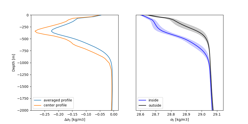
Plot anomaly

plt.figure(figsize=(10, 5))
plt.subplot(121)
plt.plot(anomaly.anomaly, anomaly.depth_vector, label="averaged profile")
plt.plot(anomaly.center_anomaly, anomaly.depth_vector, label="center profile")
plt.xlabel(r"$\Delta\sigma_0$ [kg/m3]")
# plt.xlabel(r'$\Delta cs$ [m/s]')
plt.ylabel("Depth [m]")
plt.ylim(-2000, 0)
plt.legend()
ax = plt.subplot(122)
ax.plot(anomaly.mean_profil_inside, anomaly.depth_vector, c="b", label="inside")
ax.fill_betweenx(
    anomaly.depth_vector,
    anomaly.mean_profil_inside - anomaly.std_profil_inside,
    anomaly.mean_profil_inside + anomaly.std_profil_inside,
    alpha=0.2,
    color="b",
)
ax.plot(anomaly.mean_profil_outside, anomaly.depth_vector, c="k", label="outside")
ax.fill_betweenx(
    anomaly.depth_vector,
    anomaly.mean_profil_outside - anomaly.std_profil_outside,
    anomaly.mean_profil_outside + anomaly.std_profil_outside,
    alpha=0.2,
    color="k",
)
plt.legend()
plt.xlabel(r"$\sigma_0$ [kg/m3]")
# plt.xlabel(r'$cs$ [m/s]')
# plt.ylabel('Depth [m]')
plt.yticks([], [])
plt.ylim(-2000, 0)

(-2000.0, 0.0)

Compute anomalies of all eddies

compute_anomalies(eddies, ds_3d.sig0, r_factor=1.05)